Aadhav built this feature, focusing on the backend, while Subham worked on the frontend. This article was written in collaboration with Guhan.
We recently incorporated cost dashboards and reports into Argonaut. These features are designed with the user in mind and to offer users transparency on cost matters at absolutely no extra charge. This technical blog explores the underlying layers of this feature and how we built this, starting with the tools used, retrieving and processing cost data, implementing filters for cost reports, as well as the system architecture.
Why cost visibility?
Cost visibility in cloud terms refers to the process of analyzing and visualizing your spending along with resource, account, and region-level specifics. It is crucial for businesses and teams to have a clear understanding of which resources are costing them the most. This is an essential first step to establishing good FinOps practices within your organization.
Our new cost visibility features - cost reports and cost dashboards were created to deliver holistic views of your AWS costs and, in response to managing cloud costs becoming a primary challenge for teams, as indicated by 82% of respondents in recent surveys.
Tools and technologies used
We used the following for our cost feature.
Backend:
- AWS CloudFormation (for setting up resources on users' environments)
- AWS SQS + AWS SNS (our primary message queue)
- Argo Workflows (workflow engine)
- PostgreSQL (workflow metadata persistence)
- MongoDB (for storing cost data)
- Pandas (for data processing)
UI:
- chart.js, react-chartjs-2 (for charts)
- react-date-range (for date picker)
- react-table (for constructing tables)
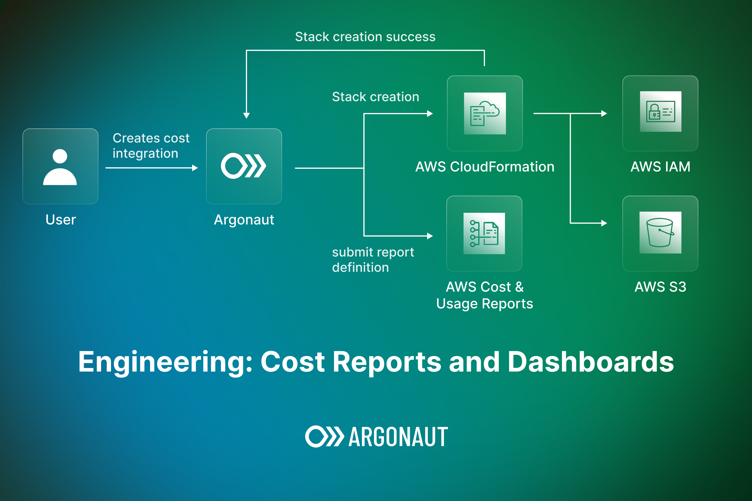
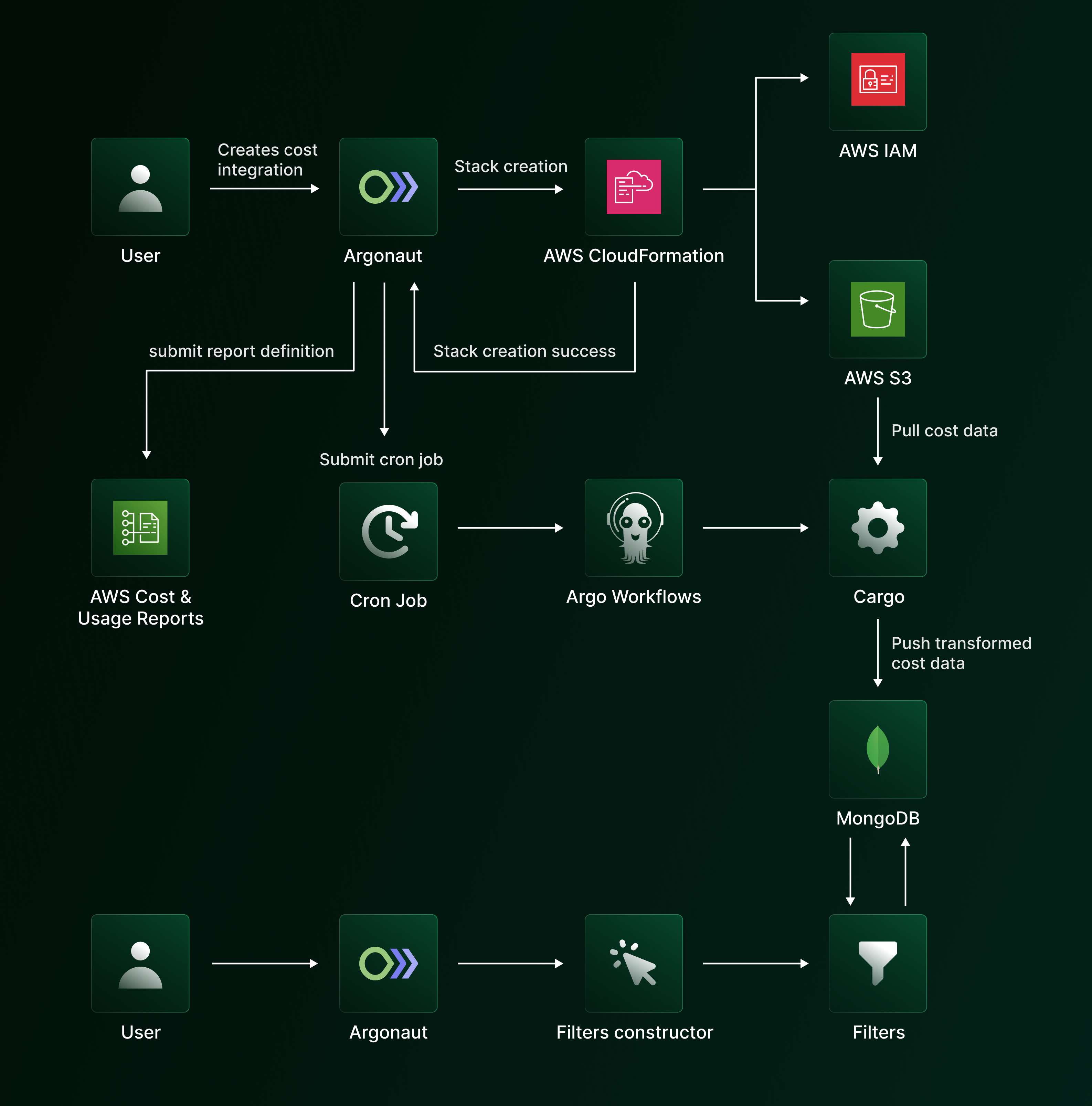
The Big Picture
Let us start with the overall architecture. As shown in the image below, we have 4 main components - stack creation, workflow submissions, data processing and filters. We will explore each of them in detail in the upcoming sections.
Getting cost data from cloud providers
As the first step, we needed to get granular billing data for each cloud resource, for example, in which region does a cluster reside in, what is the instance type for it, what is the rate for that instance type, and so on.
Thankfully, most cloud providers provide this data. In our case, AWS provides this data through Cost and Usage Reports (AWS CUR). The Cost and Usage Report is a detailed report that includes information about the usage of your AWS services, pricing, etc.
The reports are CSV files that AWS delivers to an S3 bucket which you specify while creating the report. AWS refreshes this data regularly based on the configured schedule (hourly/daily/monthly).
The generation of the first report takes around 24 hours, after which AWS will refresh data based on the configured schedule.
Setting up a few resources
In order for AWS Cost and Usage Reports to work correctly, we need to spin up a few resources on the user's AWS account.
We use AWS CloudFormation to set up a few resources when an "Infrastructure Management" connection is created on Argonaut. We decided to stick to the existing flow of using CloudFormation to setup resources.
For the “Cost Management” connection, we create an S3 bucket (one-time create) and attach a custom bucket policy as a part of the CloudFormation stack in addition to the base Argonaut resources (IAM role and event handler). The custom bucket policy is created to ensure that AWS can deliver reports correctly to the user's S3 bucket.
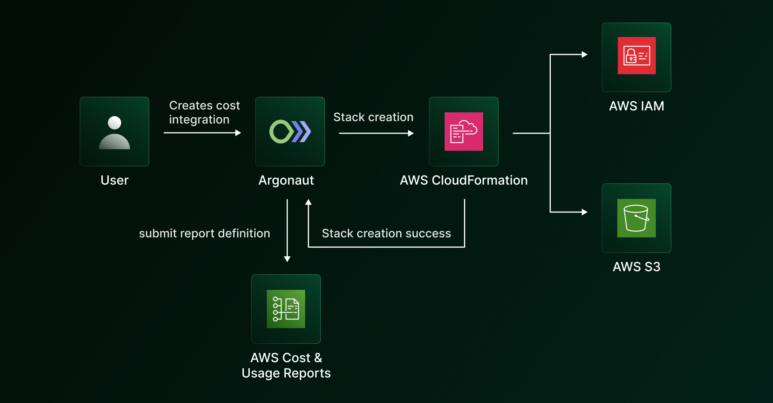
Our backend services listen for the status of the CloudFormation stack creation, and on successful creation of the stack, we trigger the creation of the Cost and Usage Report using the AWS SDK for that integration, where the bucket name is specified as the one present in the CloudFormation stack.
1// Creating a report definition on the AWS Cost and Usage Report service 2out, err := cur.costAndUsageReportService.PutReportDefinition(&costandusagereportservice.PutReportDefinitionInput{ 3 ReportDefinition: &costandusagereportservice.ReportDefinition{ 4 ReportName: aws.String(opts.ReportName), 5 S3Bucket: aws.String(opts.BucketName), 6 S3Prefix: aws.String(opts.S3Prefix), 7 TimeUnit: aws.String(opts.TimeUnit), 8 Compression: aws.String(opts.Compression), 9 Format: aws.String(opts.Format), 10 ReportVersioning: aws.String(costandusagereportservice.ReportVersioningOverwriteReport), 11 AdditionalSchemaElements: []*string{aws.String("RESOURCES")}, 12 S3Region: aws.String(opts.S3Region), 13 }, 14}) 15 16
The report gets created on AWS with the reference to the user's bucket. The report's time granularity is set to daily by default.
Synchronizing data using cronjobs
In order to pull data from users' buckets daily, we needed to set up a cron job. The cron job would run cargo (data pipeline) on a specified schedule.
Since we use Argo Workflows internally for handling workflows, we decided to use it for running cron jobs too. This builds on the good internal ecosystem built around it, and it would provide us with a single pane for visibility of both types of workloads (infrastructure and cost).
When a cost integration is created successfully, we trigger a cron workflow submission to our internal Argo Workflows instance. This gets registered in our databases, and the Argo scheduler takes care of running the workflow at the specified schedule.
One small issue here is that we cannot use a static schedule for running the workflows, as all of them would get triggered at the same time leading to increased load on our clusters.
In order to mitigate this, we implemented a mechanism where the cron schedule is computed dynamically based on the integration creation time.
1delay := 6 * time.Hour
2
3// Add the delay to the current timestamp.
4// Based on this new timestamp, we construct a cron-schedule which is the in the form:
5// <updated_timestamp_minute> <updated_timestamp_hour> * * *
6// This is to ensure that the cron job gets triggered on day 1 with some delay instead of waiting for a whole day (24 hours)
7withDelay := time.Now().Add(delay)
8
9cronSchedule := fmt.Sprintf("%d %d * * *", withDelay.Minute(), withDelay.Hour())
10
As mentioned previously, the delivery of cost data may take up to 24 hours. Since the delivery semantics of Cost and Usage Reports is not a fixed duration, we cannot assure that the data will be present at a specific time.
Instead of running the workflow directly on submission, we add a delay of 6 hours to ensure that the run happens at a time when there is a possibility of the data being present in the bucket. For some users, data might have been delivered within that 6-hour period, but for users who don't have data present in their buckets, the cron job would still run on the next day and would be able to process data successfully.
Choosing a data store
In order to perform further processing on the cost data, we needed to move the data from users' buckets to our database.
We initially considered using PostgreSQL, but it didn't seem like a correct fit as the schema for cost-related data provided by cloud providers might change in the near future, which means that we would need to be in sync with their schema changes.
This can be solved by referencing a data dictionary provided by the cloud providers, which includes metadata about each column and its type. However, this would mean that we would need to perform an additional step before dumping data into our database.
Since we didn't want schema changes to block our writes, so we decided to opt for MongoDB instead of PostgreSQL. MongoDB, being schema-on-read, allowed us to effortlessly write data to our database.
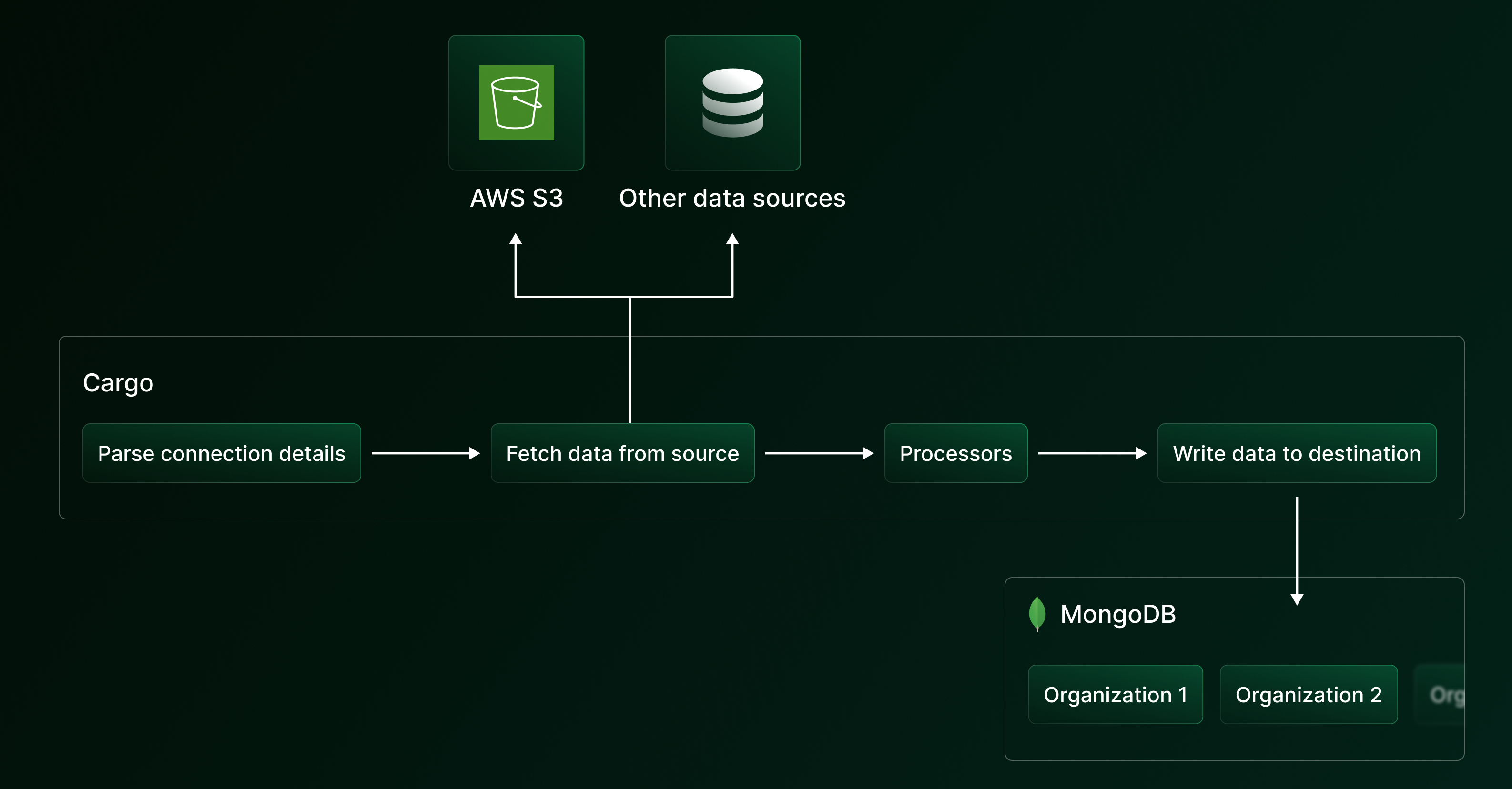
Building cargo
We built cargo, our tiny internal data pipeline written in Python for facilitating the data transfer between users' S3 buckets to our MongoDB database.
cargo is packaged as a Python CLI which accepts source and destination details as flags. Since the source and destination resource details can be different, we accept details as a string and perform parsing on top of it.
These get passed as options to our connectors, which are basically client wrappers for that resource. For example, this is how the connector factory is structured:
1class ConnectorFactory:
2
3 @staticmethod
4 def create_connector(connector_type: str, **kwargs) -> Any:
5 """
6 create_connector constructs connectors and passes kwargs to it.
7 """
8 if connector_type == "s3":
9 return S3Connector(**kwargs)
10 elif connector_type == "mongodb":
11 return MongoDBConnector(**kwargs)
12 elif connector_type == "local":
13 return LocalConnector(**kwargs)
14 else:
15 raise ValueError(f"Unsupported connector type: {connector_type}")
16
17
The connector factory is used to generate the source and destination clients:
1source_client = ConnectorFactory.create_connector( 2 source_type, **source_options 3) 4 5destination_client = ConnectorFactory.create_connector( 6 destination_type, **destination_options 7) 8 9
cargo reads CSV data into pandas dataframes for further processing. One issue with data coming from an upstream vendor is that the quality of data cannot be assured. The most common data quality issue which we encountered was the presence of NaN values in the reports. In order to fill NaN values correctly based on the data type, we use a custom processor:
1FILL_VALUES = {
2 np.number: 0,
3 object: "",
4 bool: False,
5 pd.Timestamp: pd.Timestamp("2023-01-01"),
6}
7
8def fillna_dtype(df, fill_values):
9 """
10 fillna_dtype is a wrapper around pandas' fillna for filling NaN values based on the column type.
11 """
12 # Iterate over each dtype specified in fill values
13 for dtype, fill_value in fill_values.items():
14 # Select a subset of columns matching the dtype
15 cols = df.select_dtypes(include=[dtype]).columns
16 # Fill NaN values with fill value
17 df.update(df[cols].fillna(fill_value))
18
19 return df
20
21
Once the data is loaded into the DataFrame, we write it to MongoDB in chunks:
1chunked_data = [
2 data[i : i + self.chunk_size]
3 for i in range(0, len(data), self.chunk_size)
4]
5
6progress_bar = tqdm(
7 total=len(chunked_data) * self.chunk_size
8)
9
10for chunk in chunked_data:
11 collection.insert_many(chunk)
12 progress_bar.update(self.chunk_size)
13
14progress_bar.close()
15
16
We run cargo as a part of the cron jobs running inside Argo Workflows. Each user's data is stored in a separate collection for each source. (S3, BigQuery, etc.)
Implementing dynamic filters
With the raw data now present in our MongoDB database, we needed to convert it into actionable insights. For this, we implemented a basic "filter" server on top of MongoDB, which would return data based on users' filters.
A filter is structured like this:
1// Condition is a combination of field-operator-value. 2type Condition struct { 3 Field string 4 Operator string 5 Value interface{} 6} 7 8// Rule is a combination of multiple conditions joined by the specified logical operator. 9type Rule struct { 10 Conditions []Condition 11 LogicalOperator string 12} 13 14// Filter is a combination of rules joined by a logical operator. 15type Filter struct { 16 Rules []Rule 17 LogicalOperator string 18} 19 20
The problem with filters is that they're dynamic. Users can experiment with any combination of rules and conditions. We needed a way to construct filters on-the-fly in order to provide correct data.
So, we wrote a dynamic MongoDB query constructor that would convert JSON payloads received from the frontend to actual MongoDB queries. For example, a JSON payload containing the filter:
1{
2 "start_date": "2023-07-01T00:00:00.000Z",
3 "end_date": "2023-07-31T00:00:00.000Z",
4 "filter_request": {
5 "filters": [
6 {
7 "rules": [
8 {
9 "conditions": [
10 {
11 "field": "resource_type",
12 "operator": "eq",
13 "value": "Amazon Relational Database Service"
14 }
15 ]
16 }
17 ]
18 }
19 ],
20 "group_field": "start_date",
21 "logical_operator": "and"
22 },
23 // other fields..
24}
25
26
is converted to a MongoDB query like this:
1{
2 "$and": [
3 {
4 "$and": [
5 {
6 "lineItem/UsageStartDate": {
7 "$gte": "2023-07-01T00:00:00Z"
8 }
9 },
10 {
11 "lineItem/UsageEndDate": {
12 "$lte": "2023-07-31T00:00:00Z"
13 }
14 }
15 ]
16 },
17 {
18 "lineItem/LineItemType": {
19 "$in": [
20 "Usage"
21 ]
22 }
23 },
24 {
25 "$and": [
26 {
27 "product/ProductName": {
28 "$eq": "Amazon Relational Database Service"
29 }
30 }
31 ]
32 }
33 ]
34}
35
36
The query constructor also takes care of included costs like credits, taxes, discounts, etc. by dynamically creating additional filters based on the input provided.
We encountered another challenge: we wanted this to be extensible to work with data from different cloud providers in the future. We cannot hardcode AWS-specific fields while constructing filters, as it would cause maintainability issues in the long run. The idea was to use a commons package, where we define mappings for common fields that can be present in each cloud provider’s cost data like dates, etc. The common field name is mapped to the actual column name for that provider. For example, here is the mapping for AWS:
1var ProviderCommons = map[string]ProviderColumns{ 2 "aws": { 3 Account: ProviderAccount{ 4 AccountField: "lineItem/UsageAccountId", 5 }, 6 Date: ProviderDate{ 7 StartDate: "lineItem/UsageStartDate", 8 EndDate: "lineItem/UsageEndDate", 9 Format: time.RFC3339, 10 }, 11 // other fields.. 12 } 13} 14 15
For querying data, we make use of MongoDB aggregation pipelines. Our pipeline consists of three stages:
- a
matchstage which utilizes the dynamically-created filter - a
projectstage to limit the number of fields in documents, as each document consists of 100+ fields - a
groupstage, where the group key is constructed dynamically based on the cloud provider
This pipeline is passed to the MongoDB client and executed, following which we perform a set of post-retrieval processing, which includes tasks like ignoring certain resources, etc.
Conclusion
We hope this blog gives you a sense of how the Argonaut team implemented cost dashboards and reports to provide vital cost transparency for our users.
Stay tuned as we continue to develop and introduce new features. Here’s a look at the upcoming cost management-related features we’ve got planned:
- Export cloud costs in various formats (PNG, PDF, XLSX)
- View both AWS and GCP costs
- Add third-party provider costs
- Cost saving recommendations
Try out our cost reports feature today!